Mini Term Project

Goal and Background: The goal of this project is to understand how GIS can be used to solve problems. The project requirements involved creating a spatial problem that can be solved using data and other methods in ArcGIS that we learned throughout the semester.

Methods:

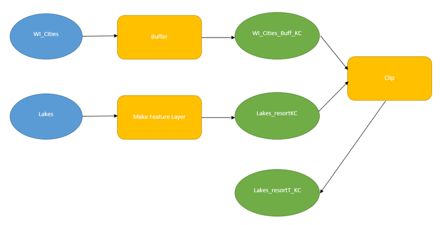
I started the process using the Select by Attributes in the WI_Counties layer to creak a feature layer of the 3 counties of study area. From there I used ArcGIS Online to get US Rivers and Streams. Minimized the area by narrowing it down to Wisconsin Rivers and Streams. I was then able to just get the Fox River when I created a layer from the selected attributes. I used a query again to Select by Attributes to get Lake Winnebago, Lake Butte des Mortes, and Lake Poygan. I included all three of the lakes to make the map more aesthetically pleasing and the lakes also connect the two halves of the Fox River.

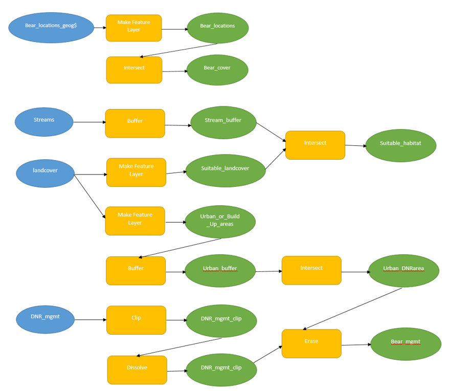
After, I downloaded the data from Geospatial Data Gateway to get National Landcover Dataset. Then I used the reclassify tool to reclassify the tiff to only Cultivated Crops. From there, I dissolved County Study Area so I could raster clip the Cultivated Crops to fit Study Area. I had to convert data from Raster to vector data so I could work with it in the map. I used Select by attributes to select all of the land that was not part of the cultivated crops (agriculture). Then I erased the non-Agriculture land from the Landover to only get Agriculture left in its own shapefile.

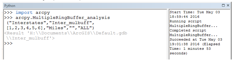
The next step included creating a multiple ring buffer around the Fox River. The intersect tool was used to put the multiple ring buffer only in the mix of land with agriculture. Erase the non-Ag land that was in the buffer. So the three rings were only shown in land that had crops.

In new data frame, WI counties and Study Area was added to act as a reference map for where the study area counties were located in Wisconsin. 

 Results:

The results of this map showed three buffer rings around the Fox River. The first one being 1.2 miles, second is 2.4 miles, and the third is 3.6 miles away from the River. The Buffer was intersected only with the Agriculture area to focus on what particular farmland was most susceptible to pollution. The first blue ring is agriculture land that produces high pollution for the river, the second pink ring is moderately hazardous, and the orange outer ring his low pollution risk to the river.

Sources:
Price Marbeth, 2016, Mastering ArcGIS, 7th Edition Data

Geospatial Data Gateway. (2016). National Landcover Dataset for Wisconsin. 

GIS I Lab 5

Goal and Background: The goal in this last lab is prove the capability of applying vector geoprocessing tools that we have learned throughout this semester and learn the how these tools work through scripting in python for ArcGIS. The objectives that need to be met include: map an excel file with GPS data; using GPS locations of black bears to determine forest types where black bears are found in Marquette County, Michigan; find bears in relation to streams habitats based on criteria; getting rid areas on that map near built up or urban land; create a model that shows the procedure used to find the bear habitat; and work with basic geoprocessing operations using python scripting

Methods:
Part 1: Bear habitat suitability modeling

Having the data model explained, you first need to create a shapefile out of the bear_locations_geog$ data in the spreadsheet. Then you intersect the bear_locations with landcover to create the bear_cover shapefile.
After that you take the streams shapefile and create a 500 m buffer around it. Then from the landcover make a layer out of the suitable_landcover. Intersect the stream_buffer and the suitable_landcover to make the suitable_habitat for the bears.
Add the DNR_mgmt shapefile to show the areas that the DNR focuses on in the county. Clip the shapefile to only get the DNG_mgmt in the study area. Dissolve the new layer to get ride of the gird areas and just have the general areas visible.
After that Use the landcover again to create a layer with Urban or Built Up Areas. Intersect the buffer around the urban areas with the DNR_mgmt that was clipped and dissolved. Then erase new shapefile with the urban buffer to create the bear management area that is within the DNR management and is also away from the Urban areas.

Part 2: Scenario 1 - Finding suitable areas for the development of tourist resorts

The model above is the data flow model of how to create the map. To find an area that is a lake that is above 5 square miles in area and also not more than 10 miles from a city. To complete the action, use the Python code that is provided in the Python box below.

Part 2: Scenario 2 -  Modeling air pollution impact zones

First, create a buffer around the interstates by typing in the Python code listed in the box below. 

When the multiple ring buffer is complete, in the symbology change the 6 names of the rings ranging from Very High to Low in distinct colors do show the 1 mile buffer zones.

Results:

This is a map of a study area that is located in Marquette County, Michigan. It includes the sustainable habitats for bears to potentially live in based on two criteria: the top three types of land, and a buffer around the streams. It shows the locations of bears and DNR management areas that are away from Urban living.

The map include the counties in which Wisconsin that have lakes that are qualified for tourist resorts. These lakes had to be greater than 5 square miles. 

In the state of Wisconsin, areas are being looked within six miles of an interstate to account for air pollution problems, suggesting that the pollution higher the closer you get to the interstate. The buffer shows six zones of potential air quality problems at one mile interval.

Sources:

Environmental Systems Research Institute. (2016).

Michigan Department of Natural Resources. (2016). Marquette County, Michigan GPS Location of Black Bears.

Price, M. (2016). Mastering ArcGIS. 7th Edition data. McGraw Hill.

Wilson, C. (2012). A comprehensive Lake features for Wisconsin. Unplublished Data.

GIS I Lab 4

Goal and Background: The goal of Lab 4 was to prove the understanding of how to use query expressions to find and use data from a particular database. The objectives included: using Boolean expressions, operators, and parenthesis to create many queries, use combination queries with attributes, and specifically map query results.


Methods: For numbers 1 through 3 (Part 1), I used the USA geodatabase from the Price mgisdata that was previously given to us. Add the counties shapefile from that geodatabase. Create a query under Selection > Select by Attributes to create the expression. The expression should include POP2010 > 3000 AND POP2010 < 4000 AND POP10_SQMI >= 1000. Create a layer from selected features to show clearly was has been selected on the map that is created of the continuous US next. Make sure the map includes Counties, Title, Legend, Map Scale and North Arrow.

For the number 2 repeat sections of number one but change the expression to (STATE_NAME = 'Wisconsin' OR STATE_NAME = 'Texas' OR STATE_NAME = 'New York' OR STATE_NAME = 'Minnesota' OR STATE_NAME = 'California') AND AGE_65_UP > 6500 AND MALES > FEMALES

Number 3 is an addition to the expression for the query in number 2. The final expression should be (STATE_NAME = 'Wisconsin' OR STATE_NAME = 'Texas' OR STATE_NAME = 'New York' OR STATE_NAME = 'Minnesota' OR STATE_NAME = 'California' OR STATE_NAME = 'Washington' OR STATE_NAME = 'Maryland' OR STATE_NAME = 'Illinois' OR STATE_NAME = 'Nebraska' OR STATE_NAME = 'District of Columbia' OR STATE_NAME = 'Michigan' ) AND AGE_65_UP > 6500 AND HSE_UNITS > 30000 AND MALES > FEMALES

Part 2 (numbers 4-5) uses the Wisconsin geodatabase that was provided. Add counties, cities, and lakes shapefile.
Number 4 asks that the query (Selection > Selection by Attributes) contains the expression POP2007 > 15000 AND POP2007 < 20000 AND AREALAND > 5 AND FEMALE > MALE. Next go to  Selection > Selection by Location and change the selection method to 'select from the currently selected features,' the target layer should be lakes and the source layer should be cities. Then make sure the spatial selection is within the distance of the source layer feature by 2 miles. Create a map of the selection which should include county, roads, and lake layers, then the title, legend, map scale, and north arrow.

Number 5 uses the counties and rivers shapefile. Use the 'Select by Attributes' again to only select the CHIPPEWA R, EAU CLAIRE R, 'EMBARRASS R, FISHER R, HUNTING R, KINNICKINNIC R, MAUNESHA R, MILWAUKEE R, MOOSE R, NAMEKAGON R, PELICAN R, PLATTE R, and POTATO R. By using the 'PNAME' = 'CHIPPEWA R' OR 'PNAME' = ... etc. for all of the selected rivers. This map should be compiled of the Wisconsin counties, major roads, lakes shapefiles and the usual map essentials.


Results:

Continuous United States showing the criteria of the population between 3,000 and 4,000 people in 2010 and all the counties that had a population density of at least 1000 persons per square mile. 

Continuous United States focusing on the states Wisconsin, Texas, New York, Minnesota, and California where the male population is greather than the female population and includes the number of seniors (age 65 and up) that is over 6,500.

Continuous United States focusing on the states Wisconsin, Texas, New York, Minnesota, and California where the male population is greather than the female population and includes the number of seniors (age 65 and up) that is over 6,500. It also adds the states Washington, Maryland, Illinois, Nebraska, D.C. and Michigan that show the seniors and counties that have more than 30,000 housing units.

Cities in Wisconsin with a population between 15,000 and 20,000 people, area of the city is at least 5 square miles in land area, female population is greater than the males, and the those cities are within 2 miles of a lake.

Only shows the Chippewa, Eau Claire, Embarrass, Fisher, Hunting, Kinnickinnic, Maunesha, Milwaukee, Moose, Namekagon, Pelican, Platte, and the Potato River in Wisconsin. 

Sources:
  Price, Maribeth H.. Mastering ArcGIS (Seventh Edition). 

GIS I Lab 3

Goal and Background: The goal of this lab was to begin obtaining GIS and other standalone data that can be used for mapping and analysis. This gives experience in shifting a standalone table containing data into an attribute table so it can be mapped. This also starts off the use of data from the U.S. Census Bureau’s website in a bid to acquire information to be used in a GIS. In the end, create a static and dynamic maps. This will be done by downloading 2010 census data from the US Census Bureau, downloading a shapefile of the 2010 Census Boundaries, joining the data to it can be mapped, build a layout with the two maps, and create a web map.

Methods:
Download data about population per Wisconsin counties and the shapefile of Wisconsin counties from 2010 US Census Bureau.
Extract the Zip files that were downloaded from the online cite.
Add the shapefile and the table to ArcMap.
Join the MS Excel file to the shapefile by joining the GEO_ID field that the two tables both have.
Create a new field labeled population and make sure it is a long integer not a string data. This way there will be values to use. Then export the data to create a new shapefile labeled Population.
Go the symbology tab. Choose quantities and graduated colors and for the value choose population. Pick a color scheme that relfects the population of Wisconsin.

Go back to the US Census Bureau and choose another variable, I chose Occupied Housing Units in 2010. Download the MS Excel file for this one as well.
Once it is downloaded and extracted, create a new layer in ArcMap. Label the Layer housing. Include the shapefile of the population used in the previous layer. Add the MS Excel file into ArcMap, and join the data to the Population shapefile.
 In the properties, change the symbology of the new feature class to display the Occupied Housing Untis. Normalize the data with population. 
Change the projection of the layer to NAD_1983_Wisconsin_TM_US_Ft
Change from the Data View to Layout view. Place the two boxes next to each other so the Population layer and the Housing layer are side by side. Add a title, Legend, north arrow, and scale to each map. 

Only using the Housing layer, change it to the WGS 1984 Web Mercator (Auxiliary sphere) coordinate system. Sign into ArcGIS Online through ArcMap under File. 

Go to Save As, Service. Then give it a name, and check Feature Access. In the left pane of the Service Editor, click Item Description and enter a summary, tags and description for the service. Analyze it so there is no errors, then share it.

Using Google Chrome browser, Sign in to ArcGIS Online (http://www.arcgis.com/home). Under My Content the map that was just uploaded will be there. Click on it,
In the drop down arrow next to the name to click on 'Add Layer to Map.' Your map should lay on top of the topographic basemap.

In the Configure Pop-up window, Change the title to Occupied Housing Units, then click on Configure Attributes. Only have Name and Population selected, also make sure they are labeled County and Population. Click OK twice. Save the map to complete the Web Map.

Results:

Static Map of Population in Wisconsin per County and Occupied Housing Units based on Population

Web/Dynamic Map of Occupied Housing units based on the population of Wisconsin in 2010.

Sources: 

American Fact Finder. (2016, January). Retrieved from US Census Bureau: http://factfinder.census.gov/faces/nav/jsf/pages/index.xhtml

Price, M. H. (2016). Mastering ArcGIS. New York: McGraw-Hill Education .

GIS 1 Lab 1

Goal and Background:  In this lab, you can recognize the differences between geographic and projected coordinate systems.  In the end, you should be able to notice projection errors, project the data so that it can be usable in GIS. The objectives include: building several data frames using feature data of different projections in the world, create a shapefile of the state of Wisconsin and apply its appropriate projection, project a data sets in different projections, then create a map that demonstrates all of the projections, and lastly, create a map of Wisconsin that includes the counties and rivers in the central area.


Methods: For the map projections each one used the country and geogrid shapefile in the World folder. In each separate each map, you changed the properties to change each Data Frame to the destined map projection. For example, the Geographic Projection Data Frame used WGS 1984. You do this for the next 4 maps. Make projections for Data Frames for Mercator Projection, Equidistant Conic, Sinusoidal, and Cylindrical Equal Area.

For the Wisconsin UTM map, you first used the states shapefile from the US folder. Go to the attributes and select the state of Wisconsin. From there, create a layer from the selected features. Export that data to create the new Wisconsin shapefile. Finally change the projection of  Wisconsin to NAD 1983 UTM Zone 16N by changing the properties of the Data Frame.

In the next Data Frame add the states shapefile again from the US folder. Next add the stroads_miv5a shapefile. Even though the shapefiles projected "on the fly," you still need to put them in the same projection. Project the stroads_miv5a shapefile to the same projection as the states shapefile by using the tool Project from the ArcToolbox. This tool is under the Data Management, then the Projections and Transformations. Save the new projected stroads_miv5a.shp. Be sure to change the Data Frame properties to the projected system in the North American Lambert Conformal Conic.

Final Data Frame will be for Central Wisconsin. Start by adding the Cenral_WI_Cts.shp. Change the Data Frame geographic coordinate system to North America_1983. Add in the Lower_Chip_strms.shp then add the same projection as the first shapefile by using the project tool. Next add scale, North Arrow, and legend. Then export the map to Adobe Illustrator. From there use the Type feature to give the map a title, label each county by it's name, and add the authors name before completing the cmap.

Results: In the figure below, this shows the different projections for the world. The Map of Wisconsin is an example of a reprojection. The projection prior to this one did not work as well as the Wisconsin UTM. And the U.S. projection involved projecting the Michigan road ways in the same projection as the U.S. projection.

The Central Wisconsin counties involved getting the rivers and counties on the same projection and the most appropriate projection for the specified area. Then I added the legend, north arrow, and scale.

Sources:

  Michigan Department of Transportation. http://www.michigan.gov/mdot/

  Price, Maribeth H.. Mastering ArcGIS (Seventh Edition).